How Much CO₂ Has Your Car Produced Since It Was Built?
Follow a car through production, years of driving and the decisions that shape its carbon history.
Illustrative scene.
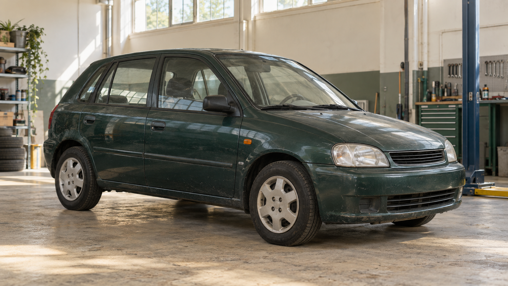
A car’s odometer keeps a record of journeys long after their details have faded. Trips to work, holidays, the years before you owned it: they all remain in that running total. For a combustion car, each stretch of distance also represents fuel that has already been burned.
Consider an illustrative petrol car with 220,000 km on the clock and an average consumption of 10.4 L/100 km. That implies 22,880 litres of fuel. Using the calculator’s mineral-petrol factor, combustion alone produces about 53.5 tonnes of CO₂. This is ATLAS arithmetic for a stated scenario, not a measurement of a particular car; it uses the separate CO₂ component in the UK government’s 2026 conversion factors.
Fuel is only part of that history. The car already carried a production footprint before its first kilometre; tyres, fluids and replacement parts add further chapters. The calculator below brings these stages together as an estimate of physical CO₂. You can follow the whole vehicle or the share assigned to your years of ownership, then explore keeping it or changing cars today.
So how much CO₂ has your car produced?
The tonnes behind the kilometres
The number may feel unexpectedly large because we usually encounter fuel in small amounts. A tankful is familiar. The sum of thousands of journeys is harder to picture.
For a combustion car, the central calculation is straightforward:
Distance × average fuel consumption ÷ 100 × CO₂ per litre.
In the example above, 220,000 × 10.4 ÷ 100 gives 22,880 litres. Multiplying by approximately 2.34 kg CO₂ per litre gives the 53.5-tonne estimate. The same method applies to diesel and LPG with their own factors; CNG is entered by mass rather than volume. The source coefficients and units are retained in the calculator’s factor table.
How can the gas weigh so much? Burning fuel joins its carbon with oxygen from the air. Much of the resulting CO₂ mass came from that oxygen. The US EPA explains this chemistry alongside its fuel-specific emissions factors. EPA: emissions from a passenger vehicle.
That is also why one generic “car emission” figure is a poor substitute for your own history. The odometer tells us how far the car travelled; consumption tells us how much fuel that distance required. A familiar model name cannot establish how it was driven, loaded or maintained.
If you have reliable long-run fuel records, use them. Otherwise, the catalogue provides a starting estimate. Applying today’s average to the whole odometer assumes that average represents earlier driving too, including previous owners. Changing that assumption changes the result.
Time turns a rate into a history
At an unchanged fuel consumption, twice the distance means twice the fuel-combustion CO₂. The timeline makes that accumulation visible. It does not mean an old car emits more per kilometre simply because it is old.
A conversion gives the history a change of direction. If a petrol car switched to LPG at 70,000 km, those first kilometres remain petrol kilometres. Gas consumption applies after the conversion, together with any petrol still used. Moving the slider back across that event changes which fuel is counted.
For LPG, the calculator starts with 20% more litres than the petrol reading: 8 L/100 km becomes 9.6 L/100 km. This is an adjustable ATLAS starting assumption, not a universal conversion factor. Replace it with the car’s actual gas consumption. Propane has less energy per litre than petrol, as the US Department of Energy explains; that general principle does not establish an exact percentage for every European LPG blend or engine. CNG uses a separate energy-equivalence starting point, with consumption in kilograms. US Department of Energy: propane fuel basics, US Alternative Fuels Data Center.
A carbon history begins before the first kilometre
At zero kilometres, no driving fuel has been counted. Yet the car has already been built.
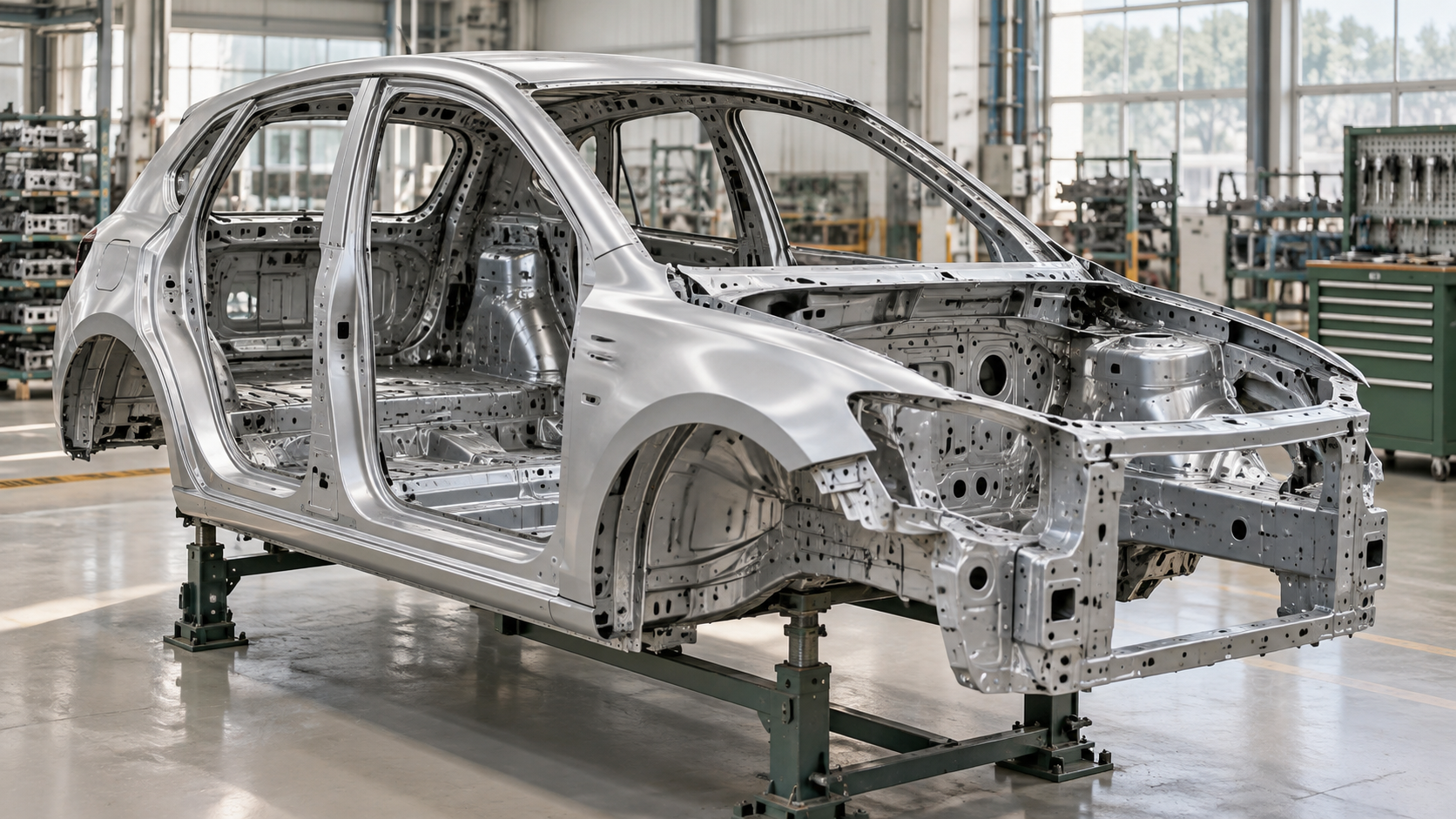
Materials had to be produced and formed, components manufactured, and the vehicle assembled. A battery adds another supply chain. Argonne’s GREET framework distinguishes this vehicle cycle from the fuel cycle: producing and using fuel does not, by itself, account for making the car. DOE’s explanation of the GREET lifecycle boundaries.
The difficulty is attaching an honest number to those earlier stages. Weight, material composition, factory energy and battery production differ between vehicles. Knowing the badge and model does not reveal the factory’s complete emissions inventory.
Illustrative scene.
The production estimate uses vehicle mass where available, historical material profiles, and process-specific CO₂ factors. Missing mass is estimated from the vehicle class. The material profiles describe broad changes in construction; they are not a factory bill of materials for your particular car. ORNL material tables, National Academies, vehicle materials.
The physical-CO₂ inventory draws on historical European material and energy processes reported in a TU Wien lifecycle study, with an older gas-resolved GREET proxy for lithium-ion batteries. These are transparent starting estimates, not modern factory measurements or an exact reconstruction of production in every model year. The factor register and limitations explain the choices. TU Wien research.
One production event, several owners
The calculator provides two views. Vehicle history counts production once, at the start of the car’s life. My ownership assigns you a share of that already-existing production footprint.
ATLAS uses a chosen ten-year allocation: 25.6%, 19.3%, 14.6%, 11.1%, 8.5%, 6.5%, 5.0%, 3.9%, 3.1% and 2.4%, starting with the first registration year. Together they distribute 100% of production. The larger early shares recognise the decision to use a newly produced vehicle, while retaining a share for subsequent owners. This is an editorial accounting convention, not an established scientific depreciation law or a mechanism by which atmospheric CO₂ disappears.
If you bought a 1994 car in 2018, no production share falls within your ownership period. Its full manufacturing emissions still appear in the vehicle’s history. If a vehicle is retired before the ten-year allocation ends, the remaining share is assigned to the final owner. Selling a car transfers its remaining scheduled shares to later years; it does not remove the car’s emissions.
Your mileage is also separate from its odometer. Buying at 100,000 km and driving another 200,000 km means 200,000 km of your travel and 300,000 km on the car. Earlier travel appears only in the vehicle-history view, with an explicit assumption where its annual distribution is unknown.
Why the average changes as you drive
For an illustrative production footprint of six tonnes of CO₂, the production component averages 60 g/km at 100,000 km and 20 g/km at 300,000 km. The six tonnes remain unchanged. Continuing to drive adds fuel or electricity emissions, so a falling average does not mean the total has fallen.
The million-kilometre explorer counts full production once and adds driving and service events. An event can cause a small upward step in emissions per kilometre. Long projections assume the vehicle remains usable; they do not predict its survival.
Servicing leaves steps in the history
Illustrative scene.
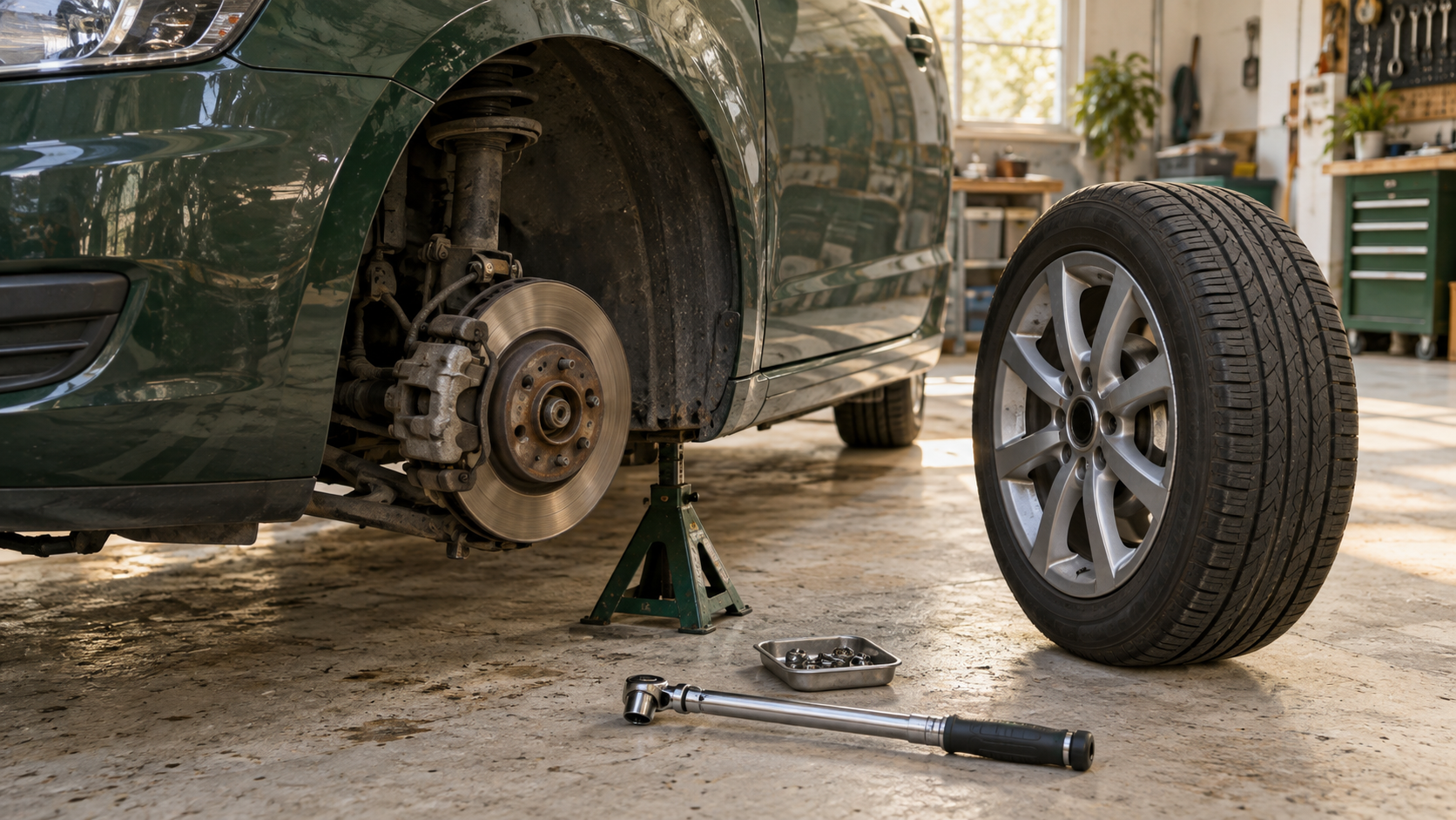
The annual bars show individual replacement events. Tyres, oil, brake parts, shock absorbers, fluids and a small auxiliary battery enter the model at specified distance or age thresholds. They are not spread into an invisible flat rate per kilometre.
These are generic schedules and assumed part quantities, not a reconstruction of your invoices. The tyre scenario uses 20,000 km as a chosen interval; real life varies. Michelin recommends age-based checks and a ten-year replacement precaution. Volkswagen’s fixed oil-service schedule provides a 15,000 km/one-year example, and Monroe provides an 80,000 km shock-absorber recommendation. None establishes a universal service schedule for every car. Michelin, Volkswagen, Monroe.
The events make timing visible, but extra detail does not guarantee extra accuracy. Workshop energy, unusual failures and major unplanned repairs are outside the current estimate.
Different fuels change the route to CO₂
Petrol, diesel, hybrid and electric cars all connect distance with energy, but they do not use the same route.
For a conventional hybrid, fuel supplies the external energy. Energy recovered during braking does not become an additional grid-electricity input. The fuel consumption already reflects the hybrid system’s effect on energy use.
A plug-in hybrid can use both fuel and electricity. Its consumption figures need particular care. Suppose it uses 6 L/100 km during fuel-powered driving, which accounts for half the distance. The fuel figure applies to that half. If your measured 3 L/100 km already covers all driving, halving it again would undercount the petrol. The calculator uses mode-specific consumption and an electric-driving distance share; do not enter an already blended figure as the fuel-mode value. Real PHEVs can also run their engine during otherwise electric driving, for example under heavy acceleration. US Department of Energy: how plug-in hybrids use fuel and electricity.
For a battery-electric car, there is no fuel-combustion CO₂ at the tailpipe. Electricity supply and vehicle production still have impacts, and appear as separate components of the estimate. EPA’s explanation of electric-vehicle emissions.
Electricity has a place, a year and a measurement point
The physical-CO₂ calculation currently uses fixed historical electricity-supply proxies for the EU, Germany, Austria and the United States. Other countries use the explicitly disclosed EU proxy. Holding the factor constant keeps the scenario reproducible, but does not capture a country’s annual grid changes or predict decarbonisation. This is a significant limitation when comparing electric vehicles across places and decades. Electricity factors and their limits.
Consumption needs a clear measurement point. A battery reading and a wall-meter reading differ because charging takes energy. Delivering 18 kWh to a battery with an assumed 10% charging loss requires 20 kWh from the wall: 18 ÷ 0.90. If the reading already comes from the charger, that loss must not be added again.
For a plug-in hybrid, enter consumption for each driving mode and the share of distance driven electrically. A blended official test value is not automatically suitable as the fuel-mode consumption.
CO₂ and CO₂e answer different questions
CO₂ is carbon dioxide. CO₂e is carbon dioxide equivalent: a common unit for comparing the warming effects of several greenhouse gases. A result of six tonnes CO₂e does not necessarily mean six tonnes of carbon dioxide were released.
The distinction matters for physical removal. Biological uptake removes CO₂; it does not directly capture the methane included in a CO₂e total. The calculator therefore uses CO₂-specific inputs for its main result. It does not multiply aggregate CO₂e data by a universal conversion ratio, and it does not imply that other gases are harmless. Methane can be particularly important for gas supply chains.
Much modern battery research reports CO₂e. For example, IVL’s 2019 update reported 61–106 kg CO₂e/kWh under its study boundaries. Those values provide climate-impact context, but are not used as kilograms of physical CO₂ in this calculator. Its older CO₂-specific battery proxy has its own substantial limitations. IVL research summary.
The same journeys, two possible futures
Choose the year you bought your car, its odometer then, and your average annual distance. The default simulation covers 15 years. Individual years can be adjusted up or down by 50%, changing the total rather than shifting kilometres into other years. A period starting in 2021 and ending at the start of 2036 contains the 15 driving years 2021–2035.
If you are considering a change today, select a new or used replacement. The calculator compares that choice with keeping the existing car, using the same future journeys and the same end date. Past ownership remains common to both scenarios. No future catalogue of cars in 2030 or 2040 is invented.
The result is your allocated footprint under the ATLAS convention. It is not a prediction of the change in global emissions caused by your purchase. Production of a new car happens up front even when its ownership shares extend over ten years. A car sold to another person can continue driving. These distinctions matter when interpreting a difference between the two totals.
What recycling can change
Finishing a simulation does not automatically scrap the car. You can continue using it, sell it or send it for recycling. Only the recycling choice activates end-of-life treatment and a potential material-recovery credit.
The credit compares recovered material with the primary material it could replace. Recovery losses, material quality, secondary processing and recycled content already credited at manufacture all affect the calculation. The current model quantifies steel and aluminium; it lists copper recovery without assigning an unsupported credit. How the recycling credit is calculated.
All credit goes to the final owner under the chosen allocation. We show gross emissions, potentially avoided emissions and the net allocated balance separately. This is a scenario comparison, not a certified offset. No historical release is erased and no atmospheric removal is claimed. EPA’s explanation of comparative recycling estimates.
How closely does this match your car?
Start with the vehicle year, then make, model and version. Check the market as well as the name. A US specification is not automatically the European version, and a registration-group average is not an exact engine or trim.
The catalogue combines EPA vehicle records, European registration data and selected manufacturer specifications. Its older European coverage is incomplete.
If your car is missing, choose “I can’t find my car”. Enter the powertrain, size class, mileage and average consumption. The size class supplies an approximate mass for the production model. It does not change a litre of fuel into a different amount of combustion CO₂.
The calculation also has boundaries beyond vehicle matching. Its fuel factors are proxies, rather than a reconstruction of the changing fuel blends bought by every owner. It excludes refrigerant leakage, roads and detailed fuel-feedstock effects. A Euro emissions class does not fill those gaps: regulated pollutants and CO₂ are different subjects. Council of the EU: Euro 7.
The calculator helps examine assumptions about keeping or replacing a car. Its allocation rule, historical process factors and simplified maintenance schedules limit what that comparison can establish; it is not an automotive recommendation.
The journeys happened. What comes next?
Return to those illustrative 53.5 tonnes of CO₂ from fuel. They describe the cumulative release implied by one car’s mileage and consumption. They are not a claim that every tonne remains in the atmosphere today: land and oceans exchange carbon with the air. IPCC: the carbon cycle.
The kilometres already happened. The fuel was already burned. Those historical emissions cannot now be prevented retroactively.
CO₂ can, however, be removed from the atmosphere. Growing trees take up CO₂ and store carbon in biomass, but meaningful removal takes real land, biological growth, management and time. Storage can also be reversed by fire, decay or other losses. A planted tree or a forecast is not the same as completed, durable removal. IPCC: carbon dioxide removal.
That is the next question at Project ATLAS: how biological uptake connects to measured carbon storage and its persistence. It begins with understanding the scale of the emissions, then examining the physical work required to remove CO₂.